Field expressions

Sometimes physical definitions of the simulation are too complex to define them with a constant value or table. To define things like material anisotropy or non-uniform field, field expressions are available in CENOS.

Field expressions applications are limited only by the imagination of the user, but a simple user guideline is still required. In this article we will look into ways on how we can define expressions and go over some of the most used applications for expressions.

How to use expressions

You can use expressions in two different ways:

• Directly - enter expression directly into the field.

• Indirectly - enter expression as Solver script and use it indirectly.

Direct definition

Choose the field of the physical value which you want to define with an expression. Then in the right part of the field change entry type from Constant to Expression, and enter your expression.

Indirect definition

You can enter the expression or value as a parameter in Solver script in Advanced computation settings and then use this parameter as an expression input in you desired field.

Expression applications

There are numerous applications on expression usage. Here we will outline the most used expression examples and provide you with an example expressions which you can copy into your simulation and alter to your liking.

Anisotropy

Many materials such as Fluxtrol have anisotropic thermal and magnetic properties, meaning that material properties depend on the direction.

equation

Tensor[X, 0, 0, 0, Y, 0, 0, 0, Z]

where X, Y and Z are the parameters in respective directions. This can be applied to any parameter such as $σ, μ$ or $λ$.

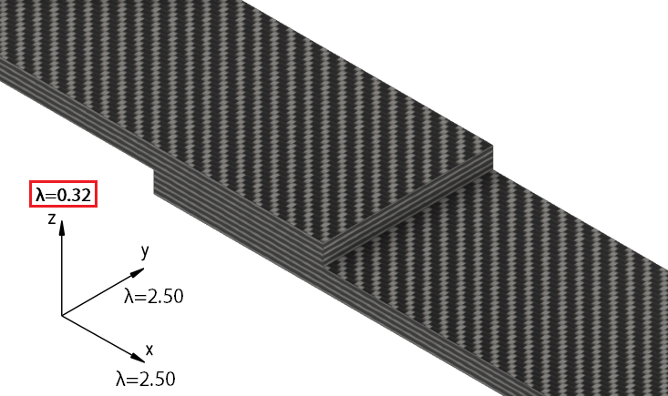
Here is an example of thermal conductivity anisotropy for a Carbon-Fiber thermoplastic piece, with a lower thermal conductivity in the Z direction. In this case we choose Expression as the parameter types and use:

Rotate anisotropy

If axis of anisotropy tensor do not align with XYZ, it is possible to rotate the tensor.

equation

Rotate [Tensor[X, 0, 0, 0, Y, 0, 0, 0, Z], Rx, Ry, Rz]

where, Rx, Ry, Rz are rotation about that axis in radians.

Example on how to rotate tensor:

equation

Rotate [ Tensor[2.50, 0, 0, 0, 2.50, 0, 0, 0, 0.32], 0, 0, 3.14/4]

In this example thermal conductivity would be maximal along the line rotated 45 degrees (pi/4 radians) around Z axis.

Global current parameter

In 3D slice multi-winding case you will have multiple winding domains which all have the same physical definitions, but which cannot be grouped because of different boundary condition names.

If you want to change the current for such simulation, you need to separately change current in each winding.

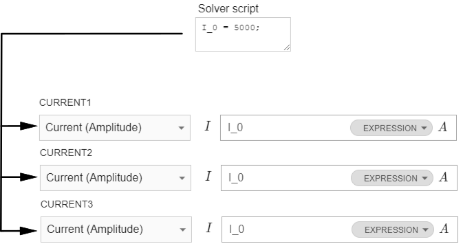
To simplify this, current can be defined in Solver script as a parameter, which can be then entered in each winding current definition. This way you will be able to change current in all windings simultaneously from Solver script.

Enter expression such as I_0 = 5000; in Solver script, and in winding current expression enter I_0. When you change the value of I_0, current values will change as well.

Moving spray cooling

In most of the induction heating scanning applications a cooling ring follows directly after the inductor, spraying cooling liquid on the workpiece and cooling it right after the heating.

With field expressions you can define a moving cooling zone to simulate spray ring which moves along with the inductor. This is done by using an expression for the convection h parameter in the workpiece domain.

equation

axis[] < y0 + velocity * $Time ? cooling_after : cooling_infront

Where:

• axis - axis of movement;
• y0 - initial spray shower position in the beginning of the movement [m];
• velocity - scanning velocity [m/s];
• cooling_behind - Heat Transfer coef. (h) value behind inductor position;
• cooling_infront - Heat Transfer coef. (h) in front of the inductor.

With this expression you define a line which is parallel to the movement axis and divides the boundary on which it has been set into two parts each with different heat transfer coefficient. When time changes, this line will change its position as well, in this way simulating the moving spray shower.

caution

Initial position and velocity values must me written in m and m/s, regardless of the unit set on the geometry.

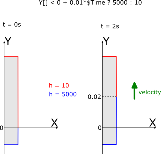
In the ilustration below you can see a simple billet with convection expression set on its surface. In the beginning of calculation (t = 0s) the dividing line is positioned on X axis (because y0 = 0), so below it h = 5000, but above it h = 10. After two seconds the line has moved 0.02m into Y direction, and now the workpiece surface division has changed and larger part of workpiece surface has h = 5000. If you imagine that in front of this line an inductor is moving, then in this way the spray cooling is simulated.

info

Moving spray cooling is not connected to the inductor movement - you define it separately and tune it to follow the inductor.

You simply need to choose the y0 value such that it follows the inductor. For example, if the inductor moves along Y axis and its initial position is Y=20mm, then for spray shower definition you would choose y0=0.01m (depending on inductor diameter).

Example:

equation

Y[] < -0.01 + 0.01 * $Time ? 5000 : 10

Where:

• Y - axis of movement;
• -0.01 m - initial spray shower position in the beginning of the movement;
• 0.01 m/s - scanning velocity;
• 5000 - Heat Transfer coef. (h) value behind inductor position;
• 10 - Heat Transfer coef. (h) in front of the inductor.

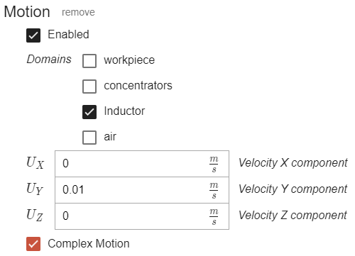
In this example the inductor is moving along Y axis. Expression puts h = 5000, if Y coordinate is smaller than y0, otherwise it puts h = 10. Notice how y0 and velocity is tuned to values which are taken from the Dynamic geometry variables - velocity remains the same (for inductor movement mm/s were used), but the y0 value is 10 mm smaller than inductors initial position to simulate the shower being behind the inductor.

Below is a comparison between different Convection definitions for the same simulation. On the left side are results with constant h = 10 (notice the excessive overheating on the surface), and on the right side is moving spray definition using expression.

Definitions for gifs below

Left : h = 10

Right : Y[] < -0.01 + 0.01$Time ? 5000 : 10

Non-uniform initial temperature

For some simulations non-uniform initial heat distribution is required. You can define such distribution through expressions by defining initial temperature as dependent from coordinate.

equation

axis[] < reference_coordinate ? T1 : T2

Where

• axis - axis of non-uniform distribution
• reference_coordinate - coordinate at which temperature changes
• T1 - temperature if coordinate is smaller than reference_coordinate
• T2 - temperature if coordinate is bigger than reference_coordinate

Which puts T = T1 if coordinate is smaller than reference_coordinate, otherwise puts T = T2.

To define non-uniform initial temperature through expression, enter it in Initial conditions field under workpiece domain.

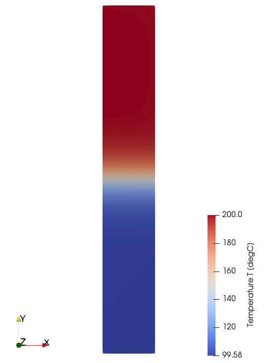
Example of non-uniform initial temperature:

equation

Y[] < 0 ? 100 : 200

In this example the temperature distribution happens along Y axis. The expression uses a temperature of 100 °C on workpiece below Y = 0 coordinate. Above it it uses a temperature of 200 °C.

Limitations

Field expressions are very useful for advanced simulation setup, but there are some things to remember to set them up correctly.

Units

Values you enter in expression, such as initial position or velocity, must be entered in meters, because that is the only unit which is supported by the expressions right now - if you enter values in other units, the expression will still work, but the value will be in meters, so the results will be incorrect.

Capital letters

Letters in field expressions are case-sensitive. For correct definition in expressions axis and other letters must be entered as capital letters, otherwise the expression will produce an error.

Correct:

Y[] < -0.01 + 0.01 * $Time ? 5000 : 10

Incorrect:

y[] < -0.01 + 0.01 * $Time ? 5000 : 10