How to estimate effective permeability (μ)
Correct material definitions within CENOS are critical for good results. One such definition is the B(H) curve, which is needed to accurately simulate the materials response to the electromagnetic field. However, the B(H) curve increases the calculation time significantly, hence it is not so effective to use during the first design iterations.
For this reason it is possible to replace the B(H) definition with a constant permeability value, which provides the same results, but in much shorter period of time.
In this article we will take a look at how to estimate the correct permeability value to use instead of a full B(H) curve.
How to find the effective μ value?
Effective permeability can be estimated by finding the maximum electric field in the workpiece. This can be done within the simulation you already have, or you can make a simplified version of your system (through symmetry, for example) to make the estimation faster.
There are two approaches to find maximum electric field H value - with and without initial B(H) calculation.
Effective μ from B(H) calculation
This approach nedds an initial simulation calculation with full B(H) material definition. The B(H) calculation will take more time, but in the end the μ estimation will be more precise.
1) Calculate the initial case with B(H)
Run one purely electromagnetic simulation of your system, without thermal analysis to decrease the calculation time.
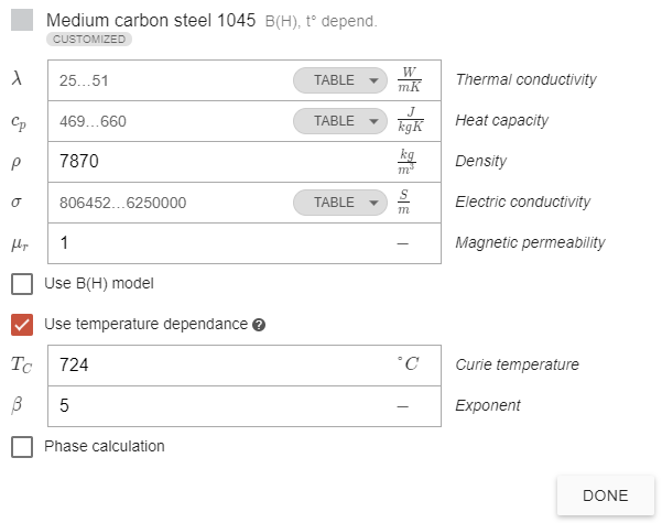
Make sure that for this test calculation you have the B(H) curve enabled for the part material, the power settings are accurate, and µ field calculation is checked in the results (to access result settings, click on the gear icon under Results block)!

![]()
2) Calculate maximum electrical field H value
Calculate the magnetic field strength through $ H = \frac{B}{μ μ_0}$ where
- – Largest magnetic field value within workpiece domain
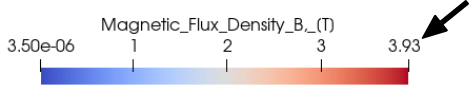
- - Lowest permeability value on the workpiece surface from results

- [H/m]
For this example:
3) Plot μ(H)
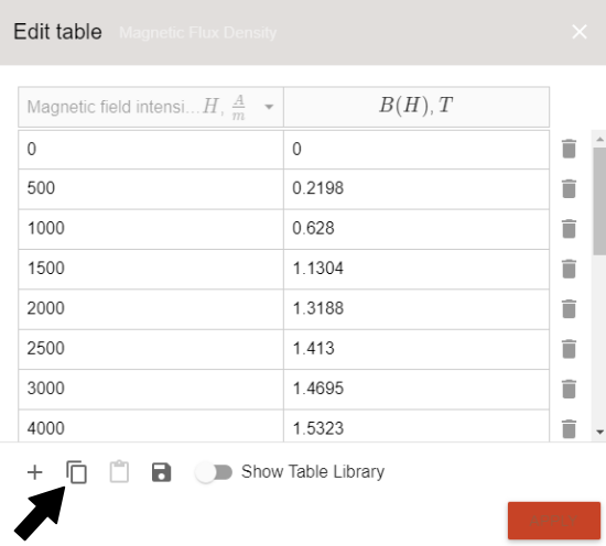
Now you need to make a µ(H) plot. Do that by first copying the B(H) definition from CENOS material properties and pasting it in MS Excel (or anywhere else).
AISI 1045 B(H) curve is used in the example.
Convert the B(H) curve to µ(H) through
(take the necessary values from the calculation done previously).
For this example we get such μ(H) graph:
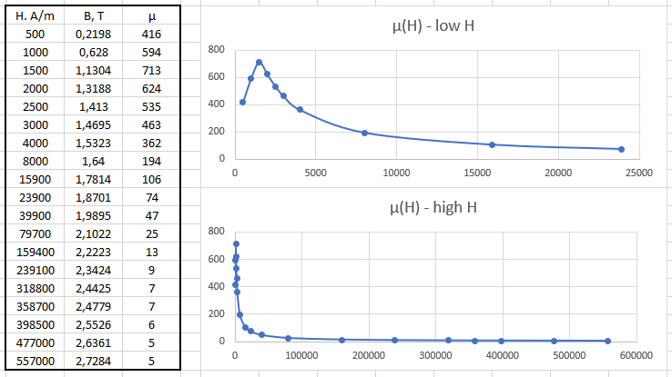
As you can see, two graphs are visualised. The upper one is to show how the permeability changes at very low H field values - it increases and then decreases in a smooth curve.
In the lower graph, where the whole H range is visualized, this initial permeability change is shown only as a spike, which is why in the full plot we cannot see the curve so clearly.
4) Read the effective μ from μ(H) plot
Once the μ(H) plot is visualized, you can read the effectve μ value corresponding to the max H value.
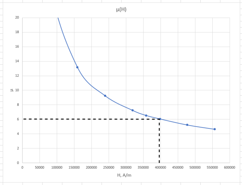
In this example the estimated effective permeability value is 6.
5) Test the estimated effective μ
Once you have estimated the effective µ, replace the B(H) curve with it in the CENOS material definition. Run the simulation with the new µ value (adjust the power if necessary).
If the result does not exactly match the one which you got with the full B(H) curve, increase or decrease the µ value and calculate some iterations until you reach the same result as with B(H) curve.
Once the results are in agreement, you have found the effective µ value, which you can use instead of B(H)!
Effective μ without B(H) calculation
This approach nedds an initial simulation calculation with workpiece material permeability defined as 1. The initial calculation will take less time, but in the end the μ estimation will help only to determine the order of μ value (1, 10, 100 etc.).
1) Define workpiece μ as 1
In CENOS disable the B(H) definition for your workpiece material and replace it with μ = 1. Make sure that the power settings are accurate!
2) Check the magnetic field B value in the workpiece
Run purely electromagnetic simulation (without thermal analysis), and in results check the maximum Magnetic field B value in the workpiece.
3) Calculate maximum electrical field H value
Calculate the maximum H value through
4) Estimate effective μ value
Once you have calculated the maximum H value, follow the steps 3. - 5. in the previous approach to estimate the effective μ value.
This method is only an approximation with high error margin, which will help to determine only the order of the μ value (1, 10, 100, etc.). If you want to have a more closer first estimation for the effective permeability, you will need to use B(H) curve approach.