Time step
There are a lot of different physical parameters, which, if defined incorrectly, can affect the precision of the results. One of such parameters with a great impact on the results is the time step. In this article we will learn what a calculation time step is, how it can affect the results and how to define it.
What is a time step?
If put simply, the calculation time step is a period of time after which the electromagnetic and thermal calculation of the simulation is done. Because of this it is quite important to correctly define the time step size, so that the calculated results would be continuous and without jumps or unphysical increases in temperature and other parameters.
How to define the time step?
Time step is defined in the physical settings under the SIMULATION CONTROL.

There are two ways on the time step definition. It is possible to define a constant calculation time step or use the adaptive time step by checking the Use adaptive time step box.
If you use constant time step, then the time step size will not change over the whole calculation time.
If adaptive time step is used, its size will automatically change from how fast the parameters such as temperature are changing.
To understand which time step definition to choose, you need to evaluate the expected results and choose the one which will provide the best accuracy.
Static heating
In case you have a static simulation, e.g. there is no movement, the temperature increase in the workpiece is usually the most rapid in the very beginning of the heating. Because of this we need to choose a time step size appropriate to resolute such fast heating.
Below are the graphs of temperature at a point on the workpiece surface from the same simulation calculated with adaptive time step and two diffrent constant time steps (0.1s and 1s).
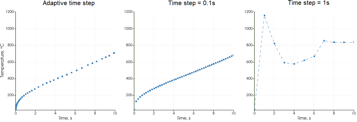
As you can see, the temperature rises very quickly in the begining, and with a rougher time step, if the heating rate is projected to the next time step, it can be unrealistically high (1200 degC).
The end temperature ir roughly similar with finer and smaller time step. However these jumps created by the rougher time step can affect the hardened profile calculation.
As you can see, even with the 0.1s time step, there is still a small jump in the temperature during the first time step. The adaptive time step resolves initial part much better, and increases the time step size further on. With adaptive there were 38 time steps, as opposed to 50 with the 0.1s time step, which means that with the adaptive step size the calculation time for this case was also lower.
Table values
If you want to resolve the initial heating better, but don't want to use Adaptive time step (to keep the control over how many time steps will be calculated), you can define the time step size in a table and make the step size smaller in the very beginning of the heating, and then increase it to save calculation time.

Scanning
If your system is not static, e.g. a translation movement is present, the time step can affect the results even more.
In a scanning simulation time step size directly affects the movement of the inductor. If the time step is too rough, inductor will "jump" from one position to another (as seen in the GIF below), making the thermal patter inconsistent and unphysical.
Because of this reason the time step should be chosen so to create a smooth movement (1 s in the example), and not to create sudden jumps in the position of it (15 s in the example).
For simple, circular-profile one-winding inductors, the neccessary time step size can be determined by considering the distance from the surface of the part to the inductor (d), as well as the distance inductor travels in one time step (Δl).

If the ratio between these two values (d and Δl) is equal or less than 1, the time step size will be enough for accurate result resolution. Below you can find a table with different d, time step size (Δt), Δl and their corresponding ratio.
