Generator efficiency

To achieve good results from your simulation it is important to input the correct parameters. When it comes to the current, voltage, or power input (depending on the system type), it is important to understand how these parameters are measured in real life and what can be used as an input for the simulation. In this article, we will look at three ways used to calculate or measure the actual power in the inductor.

Impedance matching

One of the reasons why power in the coil is lower than in the generator are the different impedance values of the load (coil) and the source (generator). Impedance is calculated as:

$$Z=\sqrt{R^2+X_L^2+X_C^2 }$$

$$X_L=2 \pi fL$$

$$X_C=\frac{1}{2 \pi fL}$$

where $L$ – inductance, $C$ – capacitance, $R$ – resistance, $f$ – frequency, $X_L$ – inductive reactance, $X_C$ – capacitive reactance.

The maximum power-transfer theorem says that to transfer the maximum amount of power from a source to a load, the load impedance should match the source impedance.

$$Z_{load} = Z_{source}$$

Find power in the generator using simulation.

Simulation can be used to estimate the efficiency of the system. To use simulation, you need to have known results from experiment, for example, the temperature on the surface of the workpiece or hardened profile of the workpiece. These results will be used as a reference to understand if the input parameters in the inductor are correct.

First, you will run a simulation with the parameters that are given on the generator. If the actual efficiency of the system is not perfect, you will see that simulation results give higher temperature values for your workpiece or hardened profile that is too wide or deep. Since the power in the simulation will be overestimated compared to reality next step is to adjust the power to get the temperature that matches the experimental results. Important: power value in the simulation can be only lower than the power in the generator.

When the power value that gives the right results is found, you can calculate the efficiency $\Gamma$ of the generator-inductor system as:

$$\Gamma=\frac{Z_{load} - Z_{source}}{Z_{load} + Z_{source}}$$

$$Z_{source} = \frac{U_{RMS}}{I_{RMS}}$$

Compare current in the generator with the current in the coil.

To measure the current in the coil you will need to use the Rogowsky coil. Rogowsky coil should be suitable for the parameters of your system such as the used current and the frequency range, they can be easily found in many internet shops. Rogowski coil is a device working on the principle that when it is placed around the inductor, the magnetic field from the inductor will induce a voltage in the coil and the converter will calculate the current in your actual inductor. Now, when setting up the simulation, you can use the measured current value in the inductor.

Voltage-controlled cases

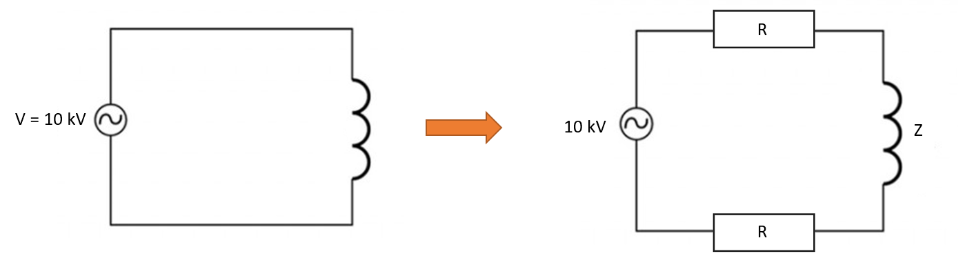
If a voltage-controlled generator is used, it means that the voltage from the generator is applied to the whole system together. The whole system is an inductor together with any kind of busbars that connects it to the generator.

Let's look at a the very simple example - a circuit with two components - generator and coil. The generator gives a constant voltage of 10 kV. The coil has its inductance L and impedance Z. That means that the voltage is constant on the whole system together, but it does not mean that the voltage is constant on the coil. We can imagine the whole system as a circuit that consists of three parts - busbar1 +inductor + busbar2. Since each busbar has its own resistance $R_1$ and $R_2$ the circuit can be re-drawn to include those.

The resistance of each busbar can be calculated

$$R=\frac{\rho l}{A}$$

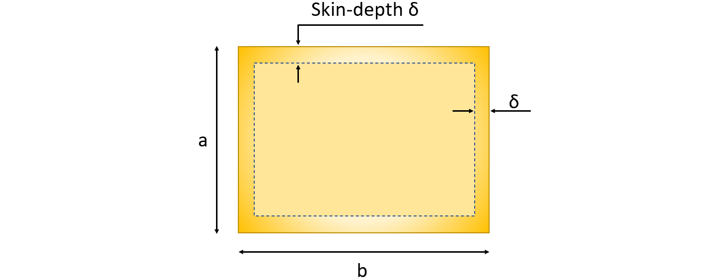
where $\rho$ is resistivity $[Ohm \cdot m]$, l – length of the busbar, A – area, where the current is flowing. To calculate area A, you need to find the skin depth in which the current is flowing and calculate this area. For example, if the inductor is rectangular with side lenght a and b, then area A is

$$A = 2 \delta a +2 \delta b - 4\delta^2$$

Each part - busbars and inductor has its own resistance. For busbars it is constant, but for the inductor part, we have to take into account its impedance which is changing in time due to the change of magnetic permeability $\mu$ of the workpiece. If we look at the total resistance of such a circuit $R_1+R_2+Z_{coil}$ it is not constant. This means that current also is not constant throughout the heating process.

$$I=\frac{V_{total}}{R_1+R_2+Z_{coil}}$$

From here we see that since the ratio between resistances $R_1 : R_2 : Z_{coil}$ is not the same all the time, the voltage drop on each part is not constant in time either. The voltage drop ratio on all three parts are the same as for the resistance $V_1 : V_2 : V_{coil}$.

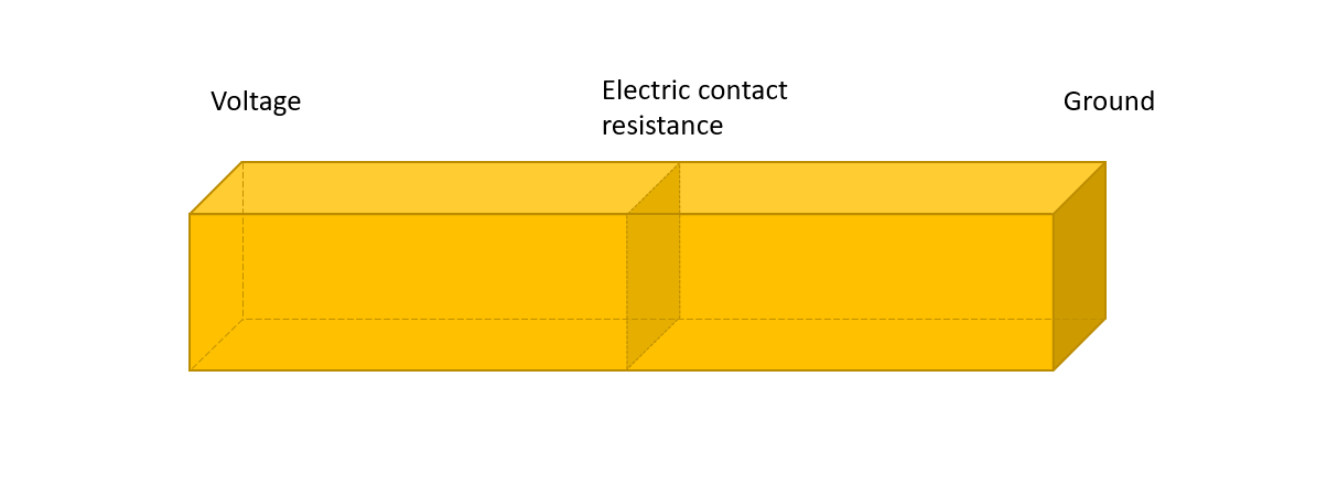
When making simulation it is important to take into account that the voltage drop is often known on the whole system, not the inductor. The workaround for this problem is to make a cut in the inductor geometry where an electric resistance boundary condition is applied. To calculate resistance

To calculate the electric constant resistance, busbar length that are left outside of simulation geometry needs to be measured. Let's say that there are two busbars with length 1.2 m, frequency used is 10 kHz, cross section of busbar is rectangle with side lengths a = 10 cm, b = 12 cm. Skin depth in this case is 652 um. To calculate area where current is flowing use equation

$$A = 2 \delta a +2 \delta b - 4\delta^2 = 2(652\cdot 10^{-6} \cdot 0.1) + 2(652 \cdot 10^{-6} \cdot 0.12) - 4(652 \cdot 10^{-6})^2 = 0.000279 m^{2}$$

Resistance of the busbars are

$$R=\frac{\rho l}{A} = \frac{1.68\cdot 10^{-8}\cdot 2\cdot 1.2}{0.000279} = 0.000145$$

Now, to calculate electric constact resistance which has units $\Omega m^2$ calculated total resistance of busbars needs to be multiplied by the cross section area of the inductor:

$$R_{contact} = R\cdot ab = 0.000145 \cdot 0.10 \cdot 0.12 = 1.74\cdot 10^{-6} \Omega m^2$$

Now, this value will represent all resistance that is not included in the simulation model but is in the real-life system.